python-[足式机器人]Part4 南科大高等机器人控制课 CH10 Bascis of Stability Analysis
推荐 原创本文仅供学习使用
本文参考:
B站:CLEAR_LAB
笔者带更新-运动学
课程主讲教师:
Prof. Wei Zhang
南科大高等机器人控制课 Ch10 Bascis of Stability Analysis
This lecture introduces basic concepts and results on Lyapunov stability of nonlinear systems
1. Background
1.1 What is Stability Analysis
- system
asymptotic/ˌæsimp'tɔtik,-kəl/ 渐进的behavior (not too much abouttransient/'trænzɪənt/短暂的) - ability to return to the desired asymptotic behavior (nout just convergence)
1.2 General ODE Models for Dynamical Systems
- ODE: x ˙ = f ( x , u ) \dot{x}=f\left( x,u \right) x˙=f(x,u) , with x ( 0 ) = x 0 x\left( 0 \right) =x_0 x(0)=x0
x ∈ X ⊆ R n x\in \mathcal{X} \subseteq \mathbb{R} ^n x∈X⊆Rn : state
u ∈ U ⊆ R m u\in \mathcal{U} \subseteq \mathbb{R} ^m u∈U⊆Rm : control input
f : R n × R m → R n f:\mathbb{R} ^n\times \mathbb{R} ^m\rightarrow \mathbb{R} ^n f:Rn×Rm→Rn : (time-invariant) vector field - System output y = g ( x , u ) y=g\left( x,u \right) y=g(x,u)
- (static)Control law : μ : X → U \mu :\mathcal{X} \rightarrow \mathcal{U} μ:X→U , u = μ ( x ) u=\mu \left( x \right) u=μ(x)
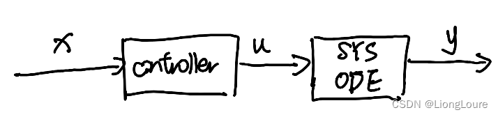
- Closed-loop dynamics under μ \mu μ : x ˙ = f ( x , μ ( x ) ) \dot{x}=f\left( x,\mu \left( x \right) \right) x˙=f(x,μ(x)) ⇒ x ˙ = f c l ( x ) \Rightarrow \dot{x}=f_{\mathrm{cl}}\left( x \right) ⇒x˙=fcl(x)
- Autonomous system :
x ˙ = f ( x , u ) \dot{x}=f\left( x,u \right) x˙=f(x,u) , with x ( 0 ) = x 0 x\left( 0 \right) =x_0 x(0)=x0
1.3 Example
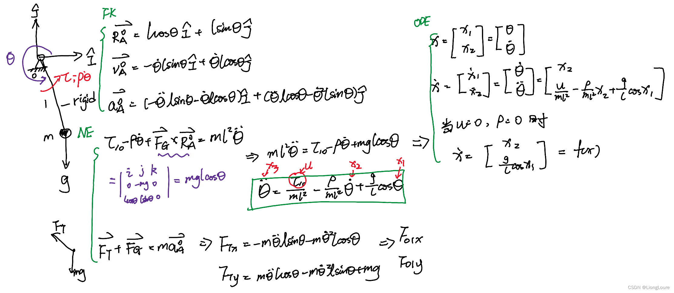
1.3.1 Pendulum
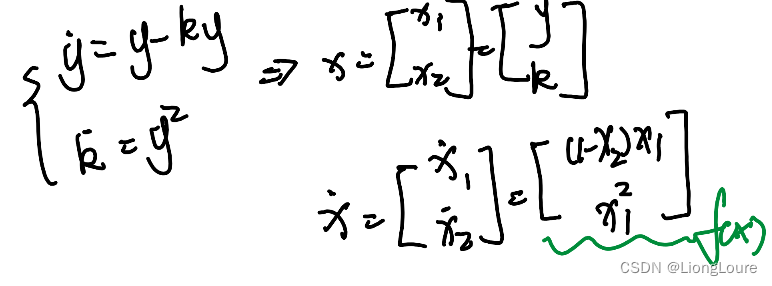
1.3.2 Adaptive Control
Closed-loop dynamics under adaptive control:
{ y ˙ = y + u u = − k y , k ˙ = y 2 \begin{cases} \dot{y}=y+u\\ u=-ky,\dot{k}=y^2\\ \end{cases} {
y˙=y+uu=−ky,k˙=y2
1.4 Equilibrium Point of Dynamical Systems
Definition 1 (Equilibrium Point) - 平衡点
A state x ∗ x^* x∗ is an equilibrium point of system (1) if once x ( t ) = x ∗ x\left( t \right) =x^* x(t)=x∗ , it remains equal to x ∗ x^* x∗ at all future time.
- Mathematically : f ( x ∗ ) = 0 f\left( x^* \right) =0 f(x∗)=0
- e.g. undamped pendulum with no driving force: f ( x ) = x ˙ f\left( x \right) =\dot{x} f(x)=x˙ velocity
x ˙ = [ x 2 g l cos x 1 ] = 0 ⇒ { x 2 = 0 cos x 1 = 0 , x 1 = 2 k π + π 2 , k ∈ Z \dot{x}=\left[ \begin{array}{c} x_2\\ \frac{g}{l}\cos x_1\\ \end{array} \right] =0\Rightarrow \begin{cases} x_2=0\\ \cos x_1=0,x_1=\frac{2k\pi +\pi}{2},k\in \mathbb{Z}\\ \end{cases} x˙=[x2lgcosx1]=0⇒{ x2=0cosx1=0,x1=22kπ+π,k∈Z
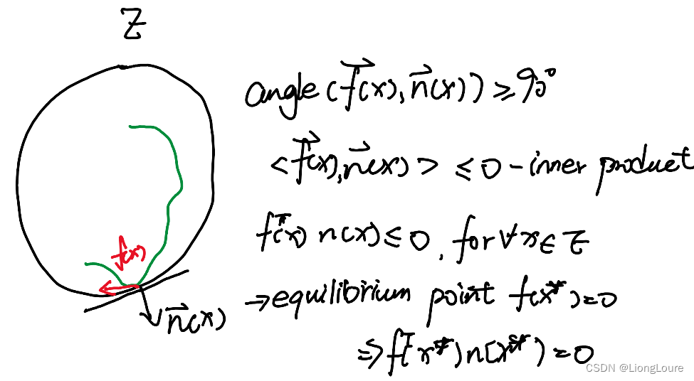
1.5 Invariant Set of Dynamical Systems
Definition 2 (Invariant Set) - 不变集
A set E E E is an invariant set of system (1) if every trajectory which starts from a point E E E remains in E E E at all future time.
- Mathematically : If x ( t 0 ) ∈ E x\left( t_0 \right) \in E x(t0)∈E , then x ( t ) ∈ E , ∀ t ⩾ t 0 x\left( t \right) \in E,\forall t\geqslant t_0 x(t)∈E,∀t⩾t0
- e.g. Closed-loop dynamics under adaptive control :
f ( x ) = x ˙ = [ x 1 − x 1 x 2 x 1 2 ] ⇒ { x 1 = 0 x 2 = a r b i t r a r y ⇒ E = { x ∈ R 2 , x 1 = 0 } f\left( x \right) =\dot{x}=\left[ \begin{array}{c} x_1-x_1x_2\\ {x_1}^2\\ \end{array} \right] \Rightarrow \begin{cases} x_1=0\\ x_2=arbitrary\\ \end{cases}\Rightarrow E=\left\{ x\in \mathbb{R} ^2,x_1=0 \right\} f(x)=x˙=[x1−x1x2x12]⇒{ x1=0x2=arbitrary⇒E={ x∈R2,x1=0}
2. Lyapunov Stability Definitions
Stability :
- about equilibrium
- ability to stay close or return to equilibrium
2.1 Lyapunov Stability Definitions
Consider a time-invariant autonomous (with no control) nonlinear system : (on closed-loop system : x ˙ = f ( x , u ( x ) ) = f c l ( x ) \dot{x}=f\left( x,u\left( x \right) \right) =f_{\mathrm{cl}}\left( x \right) x˙=f(x,u(x))=fcl(x))
x ˙ = f ( x ) , x ∈ R n \dot{x}=f\left( x \right) ,x\in \mathbb{R} ^n x˙=f(x),x∈Rn , with I.C. x ( 0 ) = x 0 x\left( 0 \right) =x_0 x(0)=x0
f ( x ) f\left( x \right) f(x) - vector field
- Assumption :
(i) f f f Lipshitz continuous —— existence & uniqueness of ODE
(ii) origin is an isolated equilibrium f ( 0 ) = 0 f\left( 0 \right) =0 f(0)=0 —— f ( x ∗ ) = 0 f\left( x^* \right) =0 f(x∗)=0
If equilibrium x ∗ x^* x∗ is not at the origin define x ~ = x − x ∗ \tilde{x}=x-x^* x~=x−x∗ , x ~ ˙ = x ˙ − 0 = f ( x ~ + x ∗ ) \dot{\tilde{x}}=\dot{x}-0=f\left( \tilde{x}+x^* \right) x~˙=x˙−0=f(x~+x∗) - Stability Definitions :
-
The equilibrium x = 0 x=0 x=0 is called stable(stay close to equilibrium) in the sense of Lyapunov , if
ϵ − δ \epsilon -\delta ϵ−δ argument —— ∀ ϵ > 0 , ∃ δ > 0 , s . t . ∥ x ( 0 ) ∥ ⩽ δ ⇒ ∥ x ( t ) ∥ ⩽ ϵ , ∀ t ⩾ 0 \forall \epsilon >0,\exists \delta >0,s.t.\left\| x\left( 0 \right) \right\| \leqslant \delta \Rightarrow \left\| x\left( t \right) \right\| \leqslant \epsilon ,\forall t\geqslant 0 ∀ϵ>0,∃δ>0,s.t.∥x(0)∥⩽δ⇒∥x(t)∥⩽ϵ,∀t⩾0
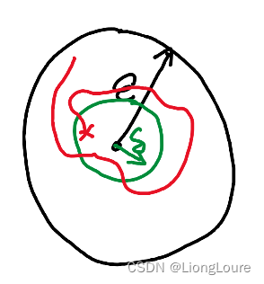
Objective: For any ϵ > 0 \epsilon >0 ϵ>0 , ensure ∥ x ( t ) ∥ ⩽ ϵ \left\| x\left( t \right) \right\| \leqslant \epsilon ∥x(t)∥⩽ϵ for all t t t
our choice : selecting initial state x ( 0 ) x\left( 0 \right) x(0)
stability : objective can be ensure by choosing I.C. sufficiently small -
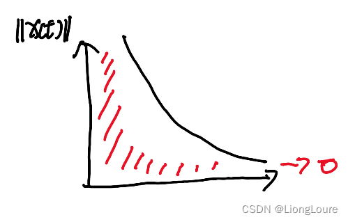
asymptotically stable (stay close + convergence) if it is stable and δ \delta δ can be chosen so that
∥ x ( 0 ) ∥ ⩽ δ ⇒ ∥ x ( t ) ∥ → 0 \left\| x\left( 0 \right) \right\| \leqslant \delta \Rightarrow \left\| x\left( t \right) \right\| \rightarrow 0 ∥x(0)∥⩽δ⇒∥x(t)∥→0 as t → ∞ t\rightarrow \infty t→∞ (convergence) -
exponentially stable if there exist positive constants δ , λ , c \delta ,\lambda ,c δ,λ,c such that
∥ x ( t ) ∥ ⩽ c ∥ x ( 0 ) ∥ e − λ t , ∀ ∥ x ( 0 ) ∥ ⩽ δ \left\| x\left( t \right) \right\| \leqslant c\left\| x\left( 0 \right) \right\| e^{-\lambda t},\forall \left\| x\left( 0 \right) \right\| \leqslant \delta ∥x(t)∥⩽c∥x(0)∥e−λt,∀∥x(0)∥⩽δ
-
globallt asymptomtotically / exponentially stable (G.A.S / G.E.S) if the above conditions holds for all δ > 0 \delta >0 δ>0
-
Region of Attraction - 吸引域 : R A ≜ { x ∈ R n : w h e v e r x ( 0 ) = x , t h e n x ( t ) → 0 } R_A\triangleq \left\{ x\in \mathbb{R} ^n:whever\,\,x\left( 0 \right) =x,then\,\,x\left( t \right) \rightarrow 0 \right\} RA≜{ x∈Rn:wheverx(0)=x,thenx(t)→0}
Globaly asymptotically stable R A ≜ R n R_A\triangleq \mathbb{R} ^n RA≜Rn
2.2 Stability Examples using 2D Phase Portrait
- Undamped pendulum with no driving force :
x ˙ = [ x 2 g l cos x 1 ] = 0 ⇒ { x 2 = 0 cos x 1 = 0 , x 1 = 2 k π + π 2 , k ∈ Z \dot{x}=\left[ \begin{array}{c} x_2\\ \frac{g}{l}\cos x_1\\ \end{array} \right] =0\Rightarrow \begin{cases} x_2=0\\ \cos x_1=0,x_1=\frac{2k\pi +\pi}{2},k\in \mathbb{Z}\\ \end{cases} x˙=[x2lgcosx1]=0⇒{ x2=0cosx1=0,x1=22kπ+π,k∈Z
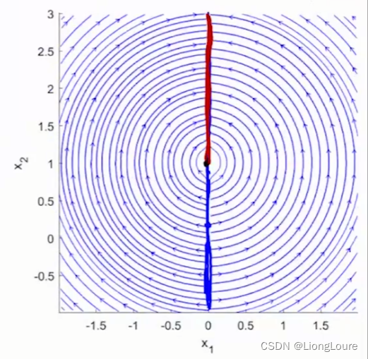
- Closed-loop dynamics under adaptive control :
f ( x ) = x ˙ = [ x 1 − x 1 x 2 x 1 2 ] ⇒ { x 1 = 0 x 2 = a r b i t r a r y ⇒ E = { x ∈ R 2 , x 1 = 0 } f\left( x \right) =\dot{x}=\left[ \begin{array}{c} x_1-x_1x_2\\ {x_1}^2\\ \end{array} \right] \Rightarrow \begin{cases} x_1=0\\ x_2=arbitrary\\ \end{cases}\Rightarrow E=\left\{ x\in \mathbb{R} ^2,x_1=0 \right\} f(x)=x˙=[x1−x1x2x12]⇒{ x1=0x2=arbitrary⇒E={ x∈R2,x1=0}
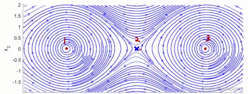
- Does attractiveness implies stable in Lyapunov sense?
Answer is No —— e.g. { x ˙ 1 = x 1 2 − x 2 2 x ˙ 2 = 2 x 1 x 2 \begin{cases} \dot{x}_1={x_1}^2-{x_2}^2\\ \dot{x}_2=2x_1x_2\\ \end{cases} { x˙1=x12−x22x˙2=2x1x2 —— asymptotically stable : 1. stable 2. convergence
By inspection of its vector field, we see that x ( t ) → 0 x\left( t \right) \rightarrow 0 x(t)→0 for all x ( 0 ) ∈ R 2 x\left( 0 \right) \in \mathbb{R} ^2 x(0)∈R2
However, there is no δ \delta δ-ball satisfying the Lyapunov stability condition
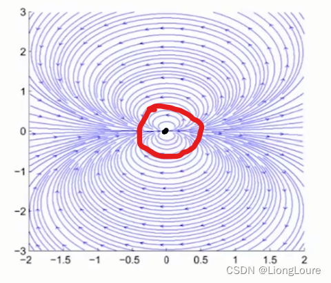
convergence but not stable
3. Lyapunov Stability Theorem
3.1 How to verify stability of a system?
- Find explicit solution of the ODE x ( t ) x\left( t \right) x(t) and check stability definitions (typically not possible for nonlinear systems) —— e.g. x ( t ) = e − t x 0 x\left( t \right) =e^{-t}x_0 x(t)=e−tx0
- Numerical simulations of ODE do not provide stability guarantees and offer limited insights
- Need to determine stability without explicitly solving the ODE
- Perferably, analysis only depends on the vector field
- The most powerful tool is : Lyapunov function
- State trajectory x ( t ) x\left( t \right) x(t) governed by complex dynamics in R n \mathbb{R} ^n Rn —— x ˙ ( t ) = f ( x ( t ) ) \dot{x}\left( t \right) =f\left( x\left( t \right) \right) x˙(t)=f(x(t))
- Lyapunov function V : R n → R V:\mathbb{R} ^n\rightarrow \mathbb{R} V:Rn→R maps x ( t ) x\left( t \right) x(t) to a scalar function of time V ( x ( t ) ) V\left( x\left( t \right) \right) V(x(t))
scalar - V ( x ( t ) ) ↔ V ˙ ( x ( t ) ) = d d t V ( x ( t ) ) = g ( V ( ) ) V\left( x\left( t \right) \right) \leftrightarrow \dot{V}\left( x\left( t \right) \right) =\frac{\mathrm{d}}{\mathrm{d}t}V\left( x\left( t \right) \right) =g\left( V\left( \right) \right) V(x(t))↔V˙(x(t))=dtdV(x(t))=g(V()) - scalar ODE - If the function is designed such that : [ x ( t ) → e q u i l i b r i u m ] ⇔ [ V ( x ( t ) ) → 0 ] \left[ x\left( t \right) \rightarrow equilibrium \right] \Leftrightarrow \left[ V\left( x\left( t \right) \right) \rightarrow 0 \right] [x(t)→equilibrium]⇔[V(x(t))→0]. Then we can study V ( x ( t ) ) V\left( x\left( t \right) \right) V(x(t)) as function of time t t t to infer stability of the state trajectory in R n \mathbb{R} ^n Rn
3.2 Sign Definite Functions
Assume that 0 ∈ D ⊆ R n 0\in D\subseteq \mathbb{R} ^n 0∈D⊆Rn
- g : D → R g:D\rightarrow \mathbb{R} g:D→R is called positive semidefinite (PSD) on D D D if g ( 0 ) = 0 g\left( 0 \right) =0 g(0)=0 and g ( 0 ) ⩾ 0 , ∀ x ∈ D g\left( 0 \right) \geqslant 0,\forall x\in D g(0)⩾0,∀x∈D
For quadratic function : g ( x ) = x T P x : [ g i s P S D ] ⇔ [ P i s a P S D m a t r i x ] g\left( x \right) =x^{\mathrm{T}}Px:\left[ g\,\,is\,\,PSD \right] \Leftrightarrow \left[ P\,\,is\,\,a\,\,PSD\,\,matrix \right] g(x)=xTPx:[gisPSD]⇔[PisaPSDmatrix]
e.g. : g ( x ) = [ x 1 x 2 ] T P [ x 1 x 2 ] = x 1 2 + x 1 x 2 + 3 x 2 2 g\left( x \right) =\left[ \begin{array}{c} x_1\\ x_2\\ \end{array} \right] ^{\mathrm{T}}P\left[ \begin{array}{c} x_1\\ x_2\\ \end{array} \right] ={x_1}^2+x_1x_2+3{x_2}^2 g(x)=[x1x2]TP[x1x2]=x12+x1x2+3x22 - g : D → R g:D\rightarrow \mathbb{R} g:D→R is called positive definite (PD) on D D D if g ( 0 ) = 0 g\left( 0 \right) =0 g(0)=0 and g ( x ) > 0 , ∀ x ∈ D \ { 0 } g\left( x \right) >0,\forall x\in D\backslash\{0\} g(x)>0,∀x∈D\{
0}
Similarly, if g ( x ) = x T P x g\left( x \right) =x^{\mathrm{T}}Px g(x)=xTPx is quadratic, then [ g i s P D ] ⇔ [ P i s a P D m a t r i x ] \left[ g\,\,is\,\,PD \right] \Leftrightarrow \left[ P\,\,is\,\,a\,\,PD\,\,matrix \right] [gisPD]⇔[PisaPDmatrix] - g g g is negative semidefinite (NSD) if − g -g −g is PSD
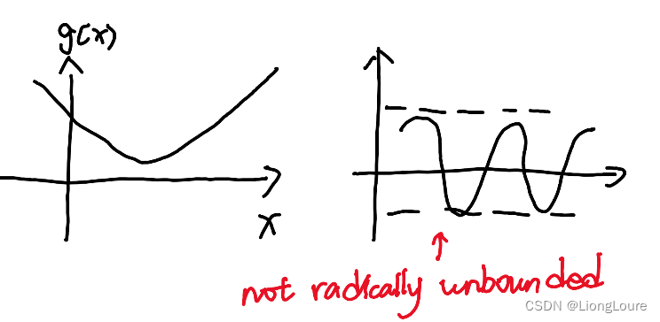
- g : R n → R g:\mathbb{R} ^n\rightarrow \mathbb{R} g:Rn→R is radically unbounded if g ( x ) → ∞ g\left( x \right) \rightarrow \infty g(x)→∞ as ∥ x ∥ → ∞ \left\| x \right\| \rightarrow \infty ∥x∥→∞
3.3 Lyapunov Stability Theorem
[Lyapunov Theorem] : Let D ⊆ R n D\subseteq \mathbb{R} ^n D⊆Rn be a set containing an open neighborhood of the origin. If there exists a C 1 \mathcal{C} ^1 C1 (continuous differentiable) function V : D → R V:D\rightarrow \mathbb{R} V:D→R (observable condition - e.g. V ( x ) = x 1 2 , x = [ x 1 x 2 ] = [ 0 100 ] , V ( x ) = 0 i s P S D V\left( x \right) ={x_1}^2,x=\left[ \begin{array}{c} x_1\\ x_2\\ \end{array} \right] =\left[ \begin{array}{c} 0\\ 100\\ \end{array} \right] \,\,,V\left( x \right) =0 is\,\,PSD V(x)=x12,x=[x1x2]=[0100],V(x)=0isPSD) such that
{ V i s P D V ˙ ( x ) ≜ ∇ V ( x ) T f ( x ) i s N S D \begin{cases} V\,\,is\,\,PD\\ \dot{V}\left( x \right) \triangleq \nabla V\left( x \right) ^{\mathrm{T}}f\left( x \right) \,\,is\,\,NSD\\ \end{cases} {
VisPDV˙(x)≜∇V(x)Tf(x)isNSD
the value of V V V along sys state trajectory nonincreasing V ˙ ( x ( t ) ) = ( ∂ V ∂ x ) T ∂ x ∂ t = ∇ V ( x ) T f ( x ) , ∇ V ( x ) [ ∂ V ∂ x 1 ∂ V ∂ x 2 ⋮ ∂ V ∂ x n ] \dot{V}\left( x\left( t \right) \right) =\left( \frac{\partial V}{\partial x} \right) ^{\mathrm{T}}\frac{\partial x}{\partial t}=\nabla V\left( x \right) ^{\mathrm{T}}f\left( x \right) ,\nabla V\left( x \right) \left[ \begin{array}{c} \frac{\partial V}{\partial x_1}\\ \frac{\partial V}{\partial x_2}\\ \vdots\\ \frac{\partial V}{\partial x_{\mathrm{n}}}\\ \end{array} \right] V˙(x(t))=(∂x∂V)T∂t∂x=∇V(x)Tf(x),∇V(x)
∂x1∂V∂x2∂V⋮∂xn∂V
, ∇ V ( x ) T f ( x ) ≜ L f [ V ] \nabla V\left( x \right) ^{\mathrm{T}}f\left( x \right) \triangleq Lf\left[ V \right] ∇V(x)Tf(x)≜Lf[V] Lie derivative of V ( ⋅ ) V\left( \cdot \right) V(⋅) with vetor field f f f
then the origin is stable. If in addition ,
V ˙ ( x ) ≜ ∇ V ( x ) T f ( x ) i s N D \dot{V}\left( x \right) \triangleq \nabla V\left( x \right) ^{\mathrm{T}}f\left( x \right) \,\,is\,\,ND V˙(x)≜∇V(x)Tf(x)isND
then the origin is asymptotically stable —— Value of V V V along sys state trajectory is decreasing
Remarks:
A PD C 1 \mathcal{C} ^1 C1 function satisfying above equation will be called a Lyapunov function (1+2 or 1+3)
Under condition 3 , if V V V is also radially unbounded —— globally asympotically stable (G.A.S)
3.4 Proof of Lyapunov Stability Theorem
Main idea : 1+2 —— stability
-
Fact : suppose V V V function satisfies 1+2 , then the sub level set Ω b ( V ) ≜ { x ∈ R n : V ( x ) ⩽ b } \varOmega _{\mathrm{b}}\left( V \right) \triangleq \left\{ x\in \mathbb{R} ^n:V\left( x \right) \leqslant b \right\} Ωb(V)≜{ x∈Rn:V(x)⩽b} is forward invariant
Proof Fact : if x ( 0 ) ∈ Ω b x\left( 0 \right) \in \varOmega _{\mathrm{b}} x(0)∈Ωb fro some b ⩾ 0 b\geqslant 0 b⩾0 , we have V ( x ( t ) ) ⩽ V ( x ( 0 ) ) ⩽ b V\left( x\left( t \right) \right) \leqslant V\left( x\left( 0 \right) \right) \leqslant b V(x(t))⩽V(x(0))⩽b ⇒ x ( t ) ∈ Ω b \Rightarrow x\left( t \right) \in \varOmega _{\mathrm{b}} ⇒x(t)∈Ωb -
Proof of stability : Given ε > 0 \varepsilon >0 ε>0 , goal is to find δ > 0 \delta >0 δ>0, such that ∥ x ( 0 ) ∥ ⩽ δ ⇒ ∥ x ( t ) ∥ ⩽ ε \left\| x\left( 0 \right) \right\| \leqslant \delta \Rightarrow \left\| x\left( t \right) \right\| \leqslant \varepsilon ∥x(0)∥⩽δ⇒∥x(t)∥⩽ε
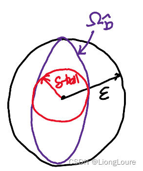
- Ω b { 0 } \varOmega _{\mathrm{b}}\left\{ 0 \right\} Ωb{ 0} if b = 0 b=0 b=0 (due to P.D. of V V V)
- As b b b increases , level set Ω b \varOmega _{\mathrm{b}} Ωb grows in size until bitting B a l l − ε Ball-\varepsilon Ball−ε then fix b = b ^ b=\hat{b} b=b^
- Find B a l l − δ Ball-\delta Ball−δ inside Ω b \varOmega _{\mathrm{b}} Ωb (because V V V is continuous at 0 0 0) then x 0 ∈ B a l l − δ ⇒ x 0 ∈ Ω b ⇒ x ( t ) ∈ Ω b x_0\in Ball-\delta \Rightarrow x_0\in \varOmega _{\mathrm{b}}\Rightarrow x\left( t \right) \in \varOmega _{\mathrm{b}} x0∈Ball−δ⇒x0∈Ωb⇒x(t)∈Ωb ( Ω b \varOmega _{\mathrm{b}} Ωb is invariant)
Sketch of proof of Lyapunov Stability theorem:
- First show stability under condition 2
Define sublevel set Ω b = { x ∈ R n : V ( x ) ⩽ b } \varOmega _{\mathrm{b}}=\left\{ x\in \mathbb{R} ^n:V\left( x \right) \leqslant b \right\} Ωb={ x∈Rn:V(x)⩽b}. Condition 2 implies V ( x ( t ) ) V\left( x\left( t \right) \right) V(x(t)) nonincreasing along system trajectory ⇒ \Rightarrow ⇒ if x 0 ∈ Ω b x_0\in \varOmega _{\mathrm{b}} x0∈Ωb , then x ( t ) ∈ Ω b x\left( t \right) \in \varOmega _{\mathrm{b}} x(t)∈Ωb, ∀ t \forall t ∀t
Given arbitrary ε > 0 \varepsilon >0 ε>0 , if we can find δ , b \delta ,b δ,b such that B ( 0 , δ ) ⊆ Ω b ⊆ B ( 0 , ε ) B\left( 0,\delta \right) \subseteq \varOmega _{\mathrm{b}}\subseteq B\left( 0,\varepsilon \right) B(0,δ)⊆Ωb⊆B(0,ε). Then the Lyapunov stability conditions are satisfied. Below is to show how we can find such b b b and δ \delta δ
V V V is continuous ⇒ \Rightarrow ⇒ m = min ∥ x ∥ = ε V ( x ) m=\min _{\left\| x \right\| =\varepsilon}V\left( x \right) m=min∥x∥=εV(x) exists (due to Weierstrass theorem). In addition, V V V is PD ⇒ \Rightarrow ⇒ m > 0 m>0 m>0. Therefore, if we choose b ∈ ( 0 , m ) b\in \left( 0,m \right) b∈(0,m) , then Ω b ⊆ B ( 0 , ε ) \varOmega _{\mathrm{b}}\subseteq B\left( 0,\varepsilon \right) Ωb⊆B(0,ε)
V ( x ) V\left( x \right) V(x) is continuous at origin ⇒ \Rightarrow ⇒ for any b > 0 b>0 b>0 , there exists δ > 0 \delta >0 δ>0 such that ∣ V ( x ) − V ( 0 ) ∣ = V ( x ) < b , ∀ x ∈ B ( 0 , δ ) \left| V\left( x \right) -V\left( 0 \right) \right|=V\left( x \right) <b,\forall x\in B\left( 0,\delta \right) ∣V(x)−V(0)∣=V(x)<b,∀x∈B(0,δ) . This implies that B ( 0 , δ ) ⊆ Ω b B\left( 0,\delta \right) \subseteq \varOmega _{\mathrm{b}} B(0,δ)⊆Ωb
- Second, show asymptotic stability under condition 3:
We know V ( x ( t ) ) V\left( x\left( t \right) \right) V(x(t)) decreases monotonically as t → ∞ t\rightarrow \infty t→∞ and V ( x ( t ) ) ⩾ 0 V\left( x\left( t \right) \right) \geqslant 0 V(x(t))⩾0, ∀ t \forall t ∀t. Therefore, c = lim t → ∞ V ( x ( t ) ) c=\lim _{t\rightarrow \infty}V\left( x\left( t \right) \right) c=limt→∞V(x(t)) exists . So it suffices to show c = 0 c=0 c=0. Let us use a contradiction argument.
Suppose c ≠ 0 c\ne 0 c=0. Then c > 0 c>0 c>0. Therefore, x ( t ) ∉ Ω c = { x ∈ R n : V ( x ) ⩽ c } x\left( t \right) \notin \varOmega _{\mathrm{c}}=\left\{ x\in \mathbb{R} ^n:V\left( x \right) \leqslant c \right\} x(t)∈/Ωc={ x∈Rn:V(x)⩽c} , ∀ t \forall t ∀t . We can choose β > 0 \beta >0 β>0 such that B ( 0 , β ) ⊆ Ω c B\left( 0,\beta \right) \subseteq \varOmega _{\mathrm{c}} B(0,β)⊆Ωc (due to continuity of V V V at 0 0 0)
Now let a = − max β ⩽ ∥ x ∥ ⩽ ε V ˙ ( x ) a=-\max _{\beta \leqslant \left\| x \right\| \leqslant \varepsilon}\dot{V}\left( x \right) a=−maxβ⩽∥x∥⩽εV˙(x). Since V V V is ND, then a > 0 a>0 a>0
V ( x ( t ) ) = V ( x ( 0 ) ) + ∫ 0 t V ˙ ( x ( s ) ) d s ⩽ V ( x ( 0 ) ) − a ⋅ t < 0 V\left( x\left( t \right) \right) =V\left( x\left( 0 \right) \right) +\int_0^t{\dot{V}\left( x\left( s \right) \right)}\mathrm{d}s\leqslant V\left( x\left( 0 \right) \right) -a\cdot t<0 V(x(t))=V(x(0))+∫0tV˙(x(s))ds⩽V(x(0))−a⋅t<0 for sufficiently large t t t. ⇒ \Rightarrow ⇒ contradiction !
3.5 Exponential Lyapunov Function
Definition 3 (Exponential Lyapunov Function) —— Important for application
V : D → R V:D\rightarrow \mathbb{R} V:D→R is called anExponential Lyapunov Function (ELF)on D ⊂ R n D\subset \mathbb{R} ^n D⊂Rn if ∃ k 1 , k 2 , k 3 , α > 0 \exists k_1,k_2,k_3,\alpha >0 ∃k1,k2,k3,α>0 such that
{ k 1 ∥ x ∥ α ⩽ V ( x ) ⩽ k 2 ∥ x ∥ α L f V ( x ) ⩽ − k 3 V ( x ) \begin{cases} k_1\left\| x \right\| ^{\alpha}\leqslant V\left( x \right) \leqslant k_2\left\| x \right\| ^{\alpha}\\ \mathcal{L} _{\mathrm{f}}V\left( x \right) \leqslant -k_3V\left( x \right)\\ \end{cases} { k1∥x∥α⩽V(x)⩽k2∥x∥αLfV(x)⩽−k3V(x)
Lyapunov stability ∃ C 1 \exists \mathcal{C} ^1 ∃C1 func V V V
V V V is PD - deserable ; V ˙ \dot{V} V˙ is ND/NSD
k 1 ∥ x ∥ α ⩽ V ( x ) ⩽ k 2 ∥ x ∥ α k_1\left\| x \right\| ^{\alpha}\leqslant V\left( x \right) \leqslant k_2\left\| x \right\| ^{\alpha} k1∥x∥α⩽V(x)⩽k2∥x∥α ⇒ V \Rightarrow V ⇒V is PD (radially unbounded)
L f V ( x ) ⩽ − k 3 V ( x ) \mathcal{L} _{\mathrm{f}}V\left( x \right) \leqslant -k_3V\left( x \right) LfV(x)⩽−k3V(x) ⇒ V ˙ \Rightarrow \dot{V} ⇒V˙ is ND, V ˙ ⩽ − k 3 V \dot{V}\leqslant -k_3V V˙⩽−k3V
Droof sketch :
recall : z ∈ R 1 , z ˙ = − k 3 z ⇒ z ( t ) = e − k 3 t z ( 0 ) z\in \mathbb{R} ^1,\dot{z}=-k_3z\Rightarrow z\left( t \right) =e^{-k_3t}z\left( 0 \right) z∈R1,z˙=−k3z⇒z(t)=e−k3tz(0)
By comparison theorem : V ˙ ⩽ − k 3 V ⇒ V ( t ) ⩽ e − k 3 t V ( 0 ) \dot{V}\leqslant -k_3V\Rightarrow V\left( t \right) \leqslant e^{-k_3t}V\left( 0 \right) V˙⩽−k3V⇒V(t)⩽e−k3tV(0)
⇒ ∥ x ( t ) ∥ α ⩽ 1 k 1 V ( x ( t ) ) ⩽ 1 k 1 e − k 3 t V ( x ( 0 ) ) ⩽ k 2 k 1 e − k 3 t ∥ x ( 0 ) ∥ α ⇒ ∥ x ( t ) ∥ α ⩽ c e − β t ∥ x ( 0 ) ∥ α \Rightarrow \left\| x\left( t \right) \right\| ^{\alpha}\leqslant \frac{1}{k_1}V\left( x\left( t \right) \right) \leqslant \frac{1}{k_1}e^{-k_3t}V\left( x\left( 0 \right) \right) \leqslant \frac{k_2}{k_1}e^{-k_3t}\left\| x\left( 0 \right) \right\| ^{\alpha}\Rightarrow \left\| x\left( t \right) \right\| ^{\alpha}\leqslant ce^{-\beta t}\left\| x\left( 0 \right) \right\| ^{\alpha} ⇒∥x(t)∥α⩽k11V(x(t))⩽k11e−k3tV(x(0))⩽k1k2e−k3t∥x(0)∥α⇒∥x(t)∥α⩽ce−βt∥x(0)∥α
Theorem 1 (ELF Theorem)
If system 2 has an ELF, then it is exponentially stable
3.6 Stability Analysis Examples
- Example 1 :
{ x ˙ 1 = − x 1 + x 2 + x 1 x 2 x ˙ 2 = x 1 − x 2 − x 1 2 − x 2 3 \begin{cases} \dot{x}_1=-x_1+x_2+x_1x_2\\ \dot{x}_2=x_1-x_2-{x_1}^2-{x_2}^3\\ \end{cases} { x˙1=−x1+x2+x1x2x˙2=x1−x2−x12−x23 Try V ( x ) = ∥ x ∥ 2 = x 1 2 + x 2 2 V\left( x \right) =\left\| x \right\| ^2={x_1}^2+{x_2}^2 V(x)=∥x∥2=x12+x22
equilibrium : x ˙ = 0 ⇒ ( x 1 x 2 ) = ( 0 0 ) \dot{x}=0\Rightarrow \left( \begin{array}{c} x_1\\ x_2\\ \end{array} \right) =\left( \begin{array}{c} 0\\ 0\\ \end{array} \right) x˙=0⇒(x1x2)=(00)
check Lyapunov conditions
- V ( x ) = x 1 2 + x 2 2 = x T [ 1 0 0 1 ] x V\left( x \right) ={x_1}^2+{x_2}^2=x^{\mathrm{T}}\left[ \begin{matrix} 1& 0\\ 0& 1\\ \end{matrix} \right] x V(x)=x12+x22=xT[1001]x is PD and C 1 \mathcal{C} ^1 C1
- L f V ( x ) = ( ∂ V ∂ x ) T f ( x ) = [ 2 x 1 2 x 2 ] T [ f 1 ( x ) f 2 ( x ) ] = 2 x 1 ( − x 1 + x 2 + x 1 x 2 ) + 2 x 2 ( x 1 − x 2 − x 1 2 − x 2 3 ) = − 2 ( x 1 − x 2 ) 2 − 2 x 2 4 ⇒ N D \mathcal{L} _{\mathrm{f}}V\left( x \right) =\left( \frac{\partial V}{\partial x} \right) ^{\mathrm{T}}f\left( x \right) =\left[ \begin{array}{c} 2x_1\\ 2x_2\\ \end{array} \right] ^{\mathrm{T}}\left[ \begin{array}{c} f_1\left( x \right)\\ f_2\left( x \right)\\ \end{array} \right] =2x_1\left( -x_1+x_2+x_1x_2 \right) +2x_2\left( x_1-x_2-{x_1}^2-{x_2}^3 \right) =-2\left( x_1-x_2 \right) ^2-2{x_2}^4\Rightarrow ND LfV(x)=(∂x∂V)Tf(x)=[2x12x2]T[f1(x)f2(x)]=2x1(−x1+x2+x1x2)+2x2(x1−x2−x12−x23)=−2(x1−x2)2−2x24⇒ND
⇒ \Rightarrow ⇒ system is asymptotically stable
- Example 2 :
{ x ˙ 1 = − x 1 + x 1 x 2 x ˙ 2 = − x 2 \begin{cases} \dot{x}_1=-x_1+x_1x_2\\ \dot{x}_2=-x_2\\ \end{cases} { x˙1=−x1+x1x2x˙2=−x2
Can we find a simple quadratic Lyapunov function ? First try V ( x ) = x 1 2 + x 2 2 V\left( x \right) ={x_1}^2+{x_2}^2 V(x)=x12+x22
- V V V is PD
- L f V ( x ) = − 2 ( ( x 2 − 4 ) 2 − 8 ) \mathcal{L} _{\mathrm{f}}V\left( x \right) =-2\left( \left( x_2-4 \right) ^2-8 \right) LfV(x)=−2((x2−4)2−8) Not ND
In fact the system does not have any (global polynomial Lyapunov function.) But it is GAS with a Lyapunov function V ( x ) = ln ( 1 + x 1 2 ) + x 2 2 V\left( x \right) =\ln \left( 1+{x_1}^2 \right) +{x_2}^2 V(x)=ln(1+x12)+x22
4. Lyapunov Stability of Linear Systems
4.1 Stability of Linear Systems
Consider autonomous linear system : x ˙ = f ( x ) = A x \dot{x}=f\left( x \right) =Ax x˙=f(x)=Ax
- Recall solution to the linear system : x ( t ) = e A t x ( 0 ) x\left( t \right) =e^{At}x\left( 0 \right) x(t)=eAtx(0)
- If isolated equilibrium only possible equilibrium is origin x = 0 x=0 x=0
f ( x ) = 0 ⇒ A x = 0 f\left( x \right) =0\Rightarrow Ax=0 f(x)=0⇒Ax=0 : 1. if A A A is nonsingular ⇒ x = 0 \Rightarrow x=0 ⇒x=0 . 2. If A A A is singular, ?? A A A is the set of equilibrium - Fact : Origin asympt. stable ⇔ \Leftrightarrow ⇔ R e ( λ i ) < 0 \mathrm{Re}\left( \lambda _{\mathrm{i}} \right) <0 Re(λi)<0 for all eigenvalues λ i \lambda _{\mathrm{i}} λi of A A A
suppose we have isolated equilibrium x ∗ = 0 x^*=0 x∗=0
For simplicity, consider a simple case when A A A is diagonalizable : A = T D T − 1 A=TDT^{-1} A=TDT−1 where D = [ λ 1 λ 2 ⋱ λ n ] D=\left[ \begin{matrix} \lambda _1& & & \\ & \lambda _2& & \\ & & \ddots& \\ & & & \lambda _{\mathrm{n}}\\ \end{matrix} \right] D= λ1λ2⋱λn ⇒ e A t = T e D t T − 1 = T [ e λ 1 t e λ 2 t ⋱ e λ n t ] T − 1 \Rightarrow e^{At}=Te^{Dt}T^{-1}=T\left[ \begin{matrix} e^{\lambda _1t}& & & \\ & e^{\lambda _2t}& & \\ & & \ddots& \\ & & & e^{\lambda _{\mathrm{n}}t}\\ \end{matrix} \right] T^{-1} ⇒eAt=TeDtT−1=T eλ1teλ2t⋱eλnt T−1 . If R e ( λ i ) < 0 \mathrm{Re}\left( \lambda _{\mathrm{i}} \right) <0 Re(λi)<0 , for all i i i , every entry of e A t → 0 e^{At}\rightarrow 0 eAt→0 ⇒ e A t x ( 0 ) \Rightarrow e^{At}x\left( 0 \right) ⇒eAtx(0) expenentially - Discrete time system : x ( k + 1 ) = A x ( k ) x\left( k+1 \right) =Ax\left( k \right) x(k+1)=Ax(k) os asymptotically stable if e i g ( A ) eig\left( A \right) eig(A) inside unit circle
4.1 Lyapunov Function of Linear Systems
- Consider a quadratic Lyapunov function candidate : V ( x ) = x T P x V\left( x \right) =x^{\mathrm{T}}Px V(x)=xTPx , with P ∈ R n × n P\in \mathbb{R} ^{n\times n} P∈Rn×n
V is PD ⇒ P ≻ 0 \Rightarrow P\succ 0 ⇒P≻0 ( P P P is a PD matrix)
L f V \mathcal{L} _{\mathrm{f}}V LfV is ND ⇒ \Rightarrow ⇒ L f V ≜ ( ∂ V ∂ x ) T A x = ( 2 P x ) T A x = 2 x T P T A x \mathcal{L} _{\mathrm{f}}V\triangleq \left( \frac{\partial V}{\partial x} \right) ^{\mathrm{T}}Ax=\left( 2Px \right) ^{\mathrm{T}}Ax=2x^{\mathrm{T}}P^{\mathrm{T}}Ax LfV≜(∂x∂V)TAx=(2Px)TAx=2xTPTAx or equirelatly, V ˙ ( x ( t ) ) = x ˙ T P x + x T P x ˙ = x T A T P x + x T P A x \dot{V}\left( x\left( t \right) \right) =\dot{x}^{\mathrm{T}}Px+x^{\mathrm{T}}P\dot{x}=x^{\mathrm{T}}A^{\mathrm{T}}Px+x^{\mathrm{T}}PAx V˙(x(t))=x˙TPx+xTPx˙=xTATPx+xTPAx —— Is 2 P T A = A T P + P A 2P^{\mathrm{T}}A=A^{\mathrm{T}}P+PA 2PTA=ATP+PA ? —— x T P T A x = x T A T P x x^{\mathrm{T}}P^{\mathrm{T}}Ax=x^{\mathrm{T}}A^{\mathrm{T}}Px xTPTAx=xTATPx
⇒ V \Rightarrow V ⇒V is LF if P P P is PD and A T P + P A A^{\mathrm{T}}P+PA ATP+PA is ND
Fact : for Linear System , quadratic form of LF , ai all we need to consider. —— A A A is asym stable if and only if ??
In proof of the above function , we assumed P P P is symmetric so P T A = P A P^{\mathrm{T}}A=PA PTA=PA
e.g. P T A = P A P^{\mathrm{T}}A=PA PTA=PA , Q = [ 1 1 − 1 1 ] , g ( x ) = x T Q x = [ x 1 x 2 ] T [ 1 1 − 1 1 ] [ x 1 x 2 ] = x 1 2 + x 2 2 ⇒ [ x 1 x 2 ] T [ 1 0 0 1 ] [ x 1 x 2 ] Q=\left[ \begin{matrix} 1& 1\\ -1& 1\\ \end{matrix} \right] , g\left( x \right) =x^{\mathrm{T}}Qx=\left[ \begin{array}{c} x_1\\ x_2\\ \end{array} \right] ^{\mathrm{T}}\left[ \begin{matrix} 1& 1\\ -1& 1\\ \end{matrix} \right] \left[ \begin{array}{c} x_1\\ x_2\\ \end{array} \right] ={x_1}^2+{x_2}^2\Rightarrow \left[ \begin{array}{c} x_1\\ x_2\\ \end{array} \right] ^{\mathrm{T}}\left[ \begin{matrix} 1& 0\\ 0& 1\\ \end{matrix} \right] \left[ \begin{array}{c} x_1\\ x_2\\ \end{array} \right] Q=[1−111],g(x)=xTQx=[x1x2]T[1−111][x1x2]=x12+x22⇒[x1x2]T[1001][x1x2] , Q ^ = 1 2 Q + 1 2 Q T \hat{Q}=\frac{1}{2}Q+\frac{1}{2}Q^{\mathrm{T}} Q^=21Q+21QT
Fact : A A A is asym stable if and only if
- ∃ P ≻ 0 \exists P\succ 0 ∃P≻0 , such that A T P + P A ≺ 0 A^{\mathrm{T}}P+PA\prec 0 ATP+PA≺0
- equivalently , for any Q ≻ 0 , ∃ P Q\succ 0,\exists P Q≻0,∃P such that A T P + P A = − Q A^{\mathrm{T}}P+PA=-Q ATP+PA=−Q (Lyapunov equation)
4.2 Stability Conditions for Linear Systems
Theorem 1 (Stability Conditions for Linear System)
For an autonomous Linear system x ˙ = A x \dot{x}=Ax x˙=Ax. The following statements are equivalent.
- (Linear) System is (globally) asmptotically stable
- (Linear) System is (globally) exponentially stable
- R e ( λ i ) < 0 \mathrm{Re}\left( \lambda _{\mathrm{i}} \right) <0 Re(λi)<0 for all eigenvalues λ i \lambda _{\mathrm{i}} λi of A A A —— lie on open left half complex plane (OLHP)
- System has a quadratic Lyapunov function V ( x ) = x T P x V\left( x \right) =x^{\mathrm{T}}Px V(x)=xTPx
- For ant symmetric Q ≻ 0 Q\succ 0 Q≻0 , there exists a symmetric P ≻ 0 P\succ 0 P≻0 that solves the following Lyapunov equation :
A T P + P A = − Q A^{\mathrm{T}}P+PA=-Q ATP+PA=−Q
Q ≻ 0 Q\succ 0 Q≻0 is given , P P P is the variale to be solved , and V ( x ) = x T P x V\left( x \right) =x^{\mathrm{T}}Px V(x)=xTPx is Lyapunov function of the system
5. Converse Lyapunov Function
When there is a Lyapunov Function?
-
Converse Lyapunov Theorem for Asymptotic Stability
origin asymptotically stable ; f f f is locallt Lipschitz on D with region of attration R A R_A RA ⇒ V s . t . \Rightarrow V\,\,s.t. ⇒Vs.t. V V V is continuuos and PD on R A R_A RA ; L f V L_{\mathrm{f}}V LfV is ND on R A R_A RA ; V ( x ) → ∞ V\left( x \right) \rightarrow \infty V(x)→∞ as x → ∂ R A x\rightarrow \partial R_{\mathrm{A}} x→∂RA
convex result that is not constructive -
Converse Lyapunov Theorem for Exponential Stability
origin exponentially stable on D D D ; f f f is C 1 \mathcal{C} ^1 C1 ⇒ ∃ \Rightarrow \exists ⇒∃ an ELF V V V on D D D -
For nonlinear sys , ∃ V ⇒ \exists V\Rightarrow ∃V⇒ stability (sufficient condition)
-
Proofs are involved especially for the converse theorem for asymptotic stability
-
Important : proofs of converse theorems often assume the knowledge of system solution and hence are not constructive
6. Extension of Discrete-Time System
6.1 What about Discrete Time Systems?
- So far, all our definitions, results, examples are given using continuous dynamical system models.
- All of them have discrete-time counterparts. The ideas and conclusions are the “same” (in sprit)
- For example, given autonomous discrete-time system : x ( k + 1 ) = f ( x ( k ) ) x\left( k+1 \right) =f\left( x\left( k \right) \right) x(k+1)=f(x(k)) with f ( 0 ) = 0 f\left( 0 \right) =0 f(0)=0 (origin is an isolated equilibrium)
Rate of change of a function V ( x ) V\left( x \right) V(x) along system trajectory can be defined as : Δ f V ( x ) = V ( f ( x ) ) − V ( x ) ⇐ V ( x ( k + 1 ) ) − V ( x ( k ) ) \varDelta _{\mathrm{f}}V\left( x \right) =V\left( f\left( x \right) \right) -V\left( x \right) \Leftarrow V\left( x\left( k+1 \right) \right) -V\left( x\left( k \right) \right) ΔfV(x)=V(f(x))−V(x)⇐V(x(k+1))−V(x(k)) , where L f V ( x ) = ( ∂ V ∂ x ) T f ( x ) L_{\mathrm{f}}V\left( x \right) =\left( \frac{\partial V}{\partial x} \right) ^{\mathrm{T}}f\left( x \right) LfV(x)=(∂x∂V)Tf(x)
Asymptotically stable requires : V V V is PD(observable all the bad behavior of ‘x’ shows up in V V V) and Δ f V \varDelta _{\mathrm{f}}V ΔfV is ND —— Δ f V ( x ) ≺ 0 \varDelta _{\mathrm{f}}V\left( x \right) \prec 0 ΔfV(x)≺0 for all x ∈ R n / { 0 } x\in \mathbb{R} ^n/\left\{ 0 \right\} x∈Rn/{ 0}
Exponentially stable requires : k 1 ∥ x ∥ α ⩽ V ( x ) ⩽ k 2 ∥ x ∥ α a n d Δ f V ( x ) ⩽ − k 3 V ( x ) k_1\left\| x \right\| ^{\alpha}\leqslant V\left( x \right) \leqslant k_2\left\| x \right\| ^{\alpha}\,\,and\,\,\varDelta _{\mathrm{f}}V\left( x \right) \leqslant -k_3V\left( x \right) k1∥x∥α⩽V(x)⩽k2∥x∥αandΔfV(x)⩽−k3V(x)
6.2 Concluding Remarks
- We have learned different notions of internal stability, e.g. stability in Lyapunov sense, asymptotic stability, globally asymptotic stability (G.A.S), exponential stability, globally exponential stability(G.E.S)
- Sufficient condition to ensure stability is often the existence of a properly defined Lyapunov function
- Key requirements for a Lyapunov function :
Positive definite and is zero at the system equilibrium
Descease along system trajectory - For linear system : G.A.S ⇔ \Leftrightarrow ⇔ G.E.S ⇔ \Leftrightarrow ⇔ Existence of a quadratic Lyapunov function
- The definitions and results in this lecture have sometimes been stated in simplified form to facilitate presentation. More general version can be found in standard textbooks on nonlinear systems
- Next Lecture : Semidefinite Programming and computational stability analysis
更多【python-[足式机器人]Part4 南科大高等机器人控制课 CH10 Bascis of Stability Analysis】相关视频教程:www.yxfzedu.com
相关文章推荐
- 前端-js实现定时刷新,并设置定时器上限 - 其他
- 需求分析-2023-11-11 事业-代号s-duck-官网首页需求分析 - 其他
- node.js-【第2章 Node.js基础】2.5 Node.js 的定时器 - 其他
- 编程技术-parasoft Jtest 使用教程:防止和检查内存问题 - 其他
- hive-【Python大数据笔记_day06_Hive】 - 其他
- 算法-【C++入门】构造函数&&析构函数 - 其他
- unity-Unity地面交互效果——4、制作地面凹陷轨迹 - 其他
- python-Django如何创建表关系,Django的请求声明周期流程图 - 其他
- 算法-力扣21:合并两个有序链表 - 其他
- 算法-Leetcode2833. 距离原点最远的点 - 其他
- node.js-Node.js中的回调地狱 - 其他
- 人工智能-AIGC(生成式AI)试用 11 -- 年终总结 - 其他
- sqlite-计算机基础知识49 - 其他
- stable diffusion-AI 绘画 | Stable Diffusion 高清修复、细节优化 - 其他
- spring-SpringBoot中的桥接模式 - 其他
- 编程技术-Halcon WPF 开发学习笔记(2):Halcon导出c#脚本 - 其他
- mysql-【MySQL】视图 - 其他
- 编程技术-1994-2021年分行业二氧化碳排放量数据 - 其他
- 编程技术-SFTP远程终端访问 - 其他
- spring-【Spring】SpringBoot配置文件 - 其他
2):严禁色情、血腥、暴力
3):严禁发布任何形式的广告贴
4):严禁发表关于中国的政治类话题
5):严格遵守中国互联网法律法规
6):有侵权,疑问可发邮件至service@yxfzedu.com